

Thailand Hydrometeorological Seasonal Forecasts
Forecasts play a crucial role in our daily lives by offering a glimpse into future conditions, helping us make informed decisions and prepare for what lies ahead. In the context of hydrometeorology, which focuses on understanding and predicting weather and water-related phenomena, forecasts are vital for anticipating weather events and their impacts. High-resolution forecasts, in particular, provide detailed and precise information that can significantly improve our ability to prepare for and respond to changing conditions. Compared with available public data, high-resolution data, such as the 1 km resolution available from our lab offers a finer, more accurate picture of localized weather patterns and hydrological events.
This level of detail is especially beneficial for sectors such as agriculture, where farmers rely on accurate weather predictions to plan their activities and protect their crops. For instance, knowing the likelihood of rainfall or temperature extremes at a very granular level allows farmers to make better decisions regarding irrigation, planting, and harvesting. Similarly, other sectors that depend on weather and water conditions—such as disaster management, infrastructure planning, and water resource management—can greatly benefit from this enhanced forecasting capability. By utilizing high-resolution data, stakeholders can improve their preparedness and response strategies, ultimately leading to more effective management of resources and risks.
Project Update:
THSF was supported by ARDA from June 2024 to June 2025. Although the project period has officially ended, we have continued providing weekly updates using funds from other sources to ensure service continuity.
Due to budget limitations, we have adjusted the processing workflow and data products to better align with our available resources. The modifications include:
- Updating the product once per month to reduce computational costs
- Reducing the number of variables to minimize storage requirements
- Providing data at a monthly temporal resolution
We will continue maintaining updates for as long as our budget allows. Thank you for your understanding and continued support.
Spatial Resolution: 0.01 equal-area grid (~1 km)
Temporal Resolution: 1 day and 1 month
Time span: 6 months forecast from present
File format: NetCDF, GeoTIFF, Excel
Latency: Once per month update
| Variable | Name | Unit | Status |
|---|---|---|---|
| AvgSurfT | Average Surface Temperature | K | Available |
| EF | Evapotranspiration Fraction | – | Discontinued |
| ESoil | Bare Soil Evaporation | gC/m²s | Discontinued |
| Evap | Evapotranspiration | kg/m²s | Available |
| GPP | Gross Primary Production | gC/m²s | Discontinued |
| GWS | Groundwater Storage | mm | Available |
| LAI | Leaf Area Index | m²/m² | Discontinued |
| Lwnet | Net Longwave Radiation | W/m² | Discontinued |
| NEE | Net Ecosystem Exchange | gC/m²s | Discontinued |
| NPP | Net Primary Production | gC/m²s | Discontinued |
| Qg | Ground Heat Flux | W/m² | Discontinued |
| Qh | Sensible Heat Flux | W/m² | Discontinued |
| Qle | Latent Heat Flux | W/m² | Discontinued |
| Qs | Surface Runoff | kg/m²s | Available |
| Qsb | Subsurface Runoff | kg/m²s | Available |
| Rainf_f | Rainfall Rate | kg/m²s | Discontinued |
| SoilMoist01 | Average layer 1 soil moisture (10 cm) | m³/m³ | Available |
| SoilMoist02 | Average layer 2 soil moisture (30 cm) | m³/m³ | Discontinued |
| SoilMoist03 | Average layer 3 soil moisture (60 cm) | m³/m³ | Discontinued |
| SoilMoist04 | Average layer 4 soil moisture (100 cm) | m³/m³ | Discontinued |
| SoilTemp01 | Average layer 1 soil temperature (10 cm) | K | Discontinued |
| SoilTemp02 | Average layer 2 soil temperature (30 cm) | K | Discontinued |
| SoilTemp03 | Average layer 3 soil temperature (60 cm) | K | Discontinued |
| SoilTemp04 | Average layer 4 soil temperature (100 cm) | K | Discontinued |
| Swnet | Net Shortwave Radiation | W/m² | Discontinued |
| Tair_f | Air Temperature | K | Discontinued |
| TVeg | Vegetation Transpiration | kg/m²s | Discontinued |
| TWS | Terrestrial Water Storage | mm | Available |
This dataset is provided for free, without any charge, as part of the provider’s commitment to the development of knowledge and collaboration in science. Registration helps users understand the scope and impact of data usage and helps the provider prioritize improvements in the future.
To access, download, or use this dataset, please Log In or Register to proceed.
The data from the Thailand Seasonal Hydro-Meteorological Forecast System (THSF) is presented in various formats. Raster data is provided in NetCDF and GeoTIFF formats for spatial analysis. Time series data is provided in Excel format, suitable for studies at basin, province, or district level. The data is updated every month and includes forecasts for the upcoming 6-month season.


Figure 1: High-resolution hydrometeorological forecast provides comprehensive variables 6 months in advance, giving a clear, localized view of changes and offering valuable insights for agriculture, water resource management, climate studies, and other sectors. This level of detail enhances the ability to make informed decisions and apply forecasts effectively at a local scale.
Instruction
You can view the instructions by clicking on any image above or by using the green buttons below. When you click, the detailed content will appear right below without leaving the page. Feel free to explore each section at your own pace!


How to register/log in/download
Our data is completely free to use, but registration is required to access downloads. This tutorial walks you through the simple registration process with screenshots at each step to ensure a smooth experience for all users, regardless of technical background.
To create an account go to:
- Log in
- Registration
📋 Step to register:
- Enter your full name/surname
- Provide your email address
- Create a password
- Input your organization name
✅ Agree to our terms of use by ticking the checkbox
Next, click “Submit” and the system will send a verification email to the address you provided. This email typically arrives within a few minutes but may take longer depending on your email provider.
After verifying your email address to activate your account, you’ll be able to navigate the platform to find and download the datasets you need.
| Variable | Description | Unit | NetCDF | GeoTiff | Figure | Excel |
|---|---|---|---|---|---|---|
| AvgSurfT | Average Surface Temperature | °C | download | download | download | download |
| EF | Evapotranspiration Fraction | - | download | download | download | download |
| ESoil | Soil Evaporation | mm/day | download | download | download | download |
| Evap | Evapotranspiration | mm/day | download | download | download | download |
| GPP | Gross Primary Production | gC/m2/day | download | download | download | download |
| GWS | Groundwater Storage | mm | download | download | download | download |
| LAI | Leaf Area Index | - | download | download | download | download |
| LWdown_f | Downward Longwave Radiation | W/m2 | download | download | download | download |
| Lwnet | Net Longwave Radiation | W/m2 | download | download | download | download |
| NEE | Net Ecosystem Exchange | gC/m2/day | download | download | download | download |
| NPP | Net Primary Production | gC/m2/day | download | download | download | download |
| Qair_f | Specific Humidity | kg/kg | download | download | download | download |
| Qg | Ground Heat Flux | W/m2 | download | download | download | download |
| Qh | Sensible Heat Flux | W/m2 | download | download | download | download |
| Qle | Latent Heat Flux | W/m2 | download | download | download | download |
| Qs | Surface Runoff | mm/day | download | download | download | download |
| Qsb | Subsurface Runoff | mm/day | download | download | download | download |
| Rainf_f | Rainfall Rate | mm/day | download | download | download | download |
| SoilMoist01 | Soil Moisture (Layer 1) | m3/m3 | download | download | download | download |
| SoilMoist02 | Soil Moisture (Layer 2) | m3/m3 | download | download | download | download |
| SoilMoist03 | Soil Moisture (Layer 3) | m3/m3 | download | download | download | download |
| SoilMoist04 | Soil Moisture (Layer 4) | m3/m3 | download | download | download | download |
| SoilTemp01 | Soil Temperature (Layer 1) | °C | download | download | download | download |
| SoilTemp02 | Soil Temperature (Layer 2) | °C | download | download | download | download |
| SoilTemp03 | Soil Temperature (Layer 3) | °C | download | download | download | download |
| SoilTemp04 | Soil Temperature (Layer 4) | °C | download | download | download | download |
| SWdown_f | Downward Shortwave Radiation | W/m2 | download | download | download | download |
| Swnet | Net Shortwave Radiation | W/m2 | download | download | download | download |
| Tair_f | Air Temperature | °C | download | download | download | download |
| TVeg | Vegetation Transpiration | mm/day | download | download | download | download |
| TWS | Terrestrial Water Storage | mm | download | download | download | download |
Remark: “Only average surface temperature (AvgSurT) data is available for use in example instructions.”
How to process data using GEE
This instructional module explores three distinct approaches for data processing within Google Earth Engine. It provides detailed guidance on utilising the GEE Code Editor for browser-based analysis, integrating Google Colab for notebook-based workflows, and employing the Python API for programming applications. Each segment includes practical code examples and use cases, enabling users to harness the computational capabilities of GEE effectively.
- GEE Setup
- GEE Editor
- Google Colab
- Python API
Google Earth Engine Access and Usage Guide
Google Earth Engine (GEE) is a cloud-based platform that enables users to analyse and visualise geospatial data at planetary scale. It provides access to a multi-petabyte catalog of satellite imagery and geospatial datasets, with tools to analyse and visualise that data.
GEE is particularly useful for:
- Environmental monitoring
- Land use and land cover mapping
- Climate research
- Disaster response
- Agricultural analysis
- Urban planning

1. Getting Started with Google Earth Engine
Sign up for GEE access:
- Visit Google Earth Engine signup page
- Use your Google account to register
- Select whether you’ll use GEE for research, education, or non-profit work
- Wait for approval (usually takes 1-2 business days)


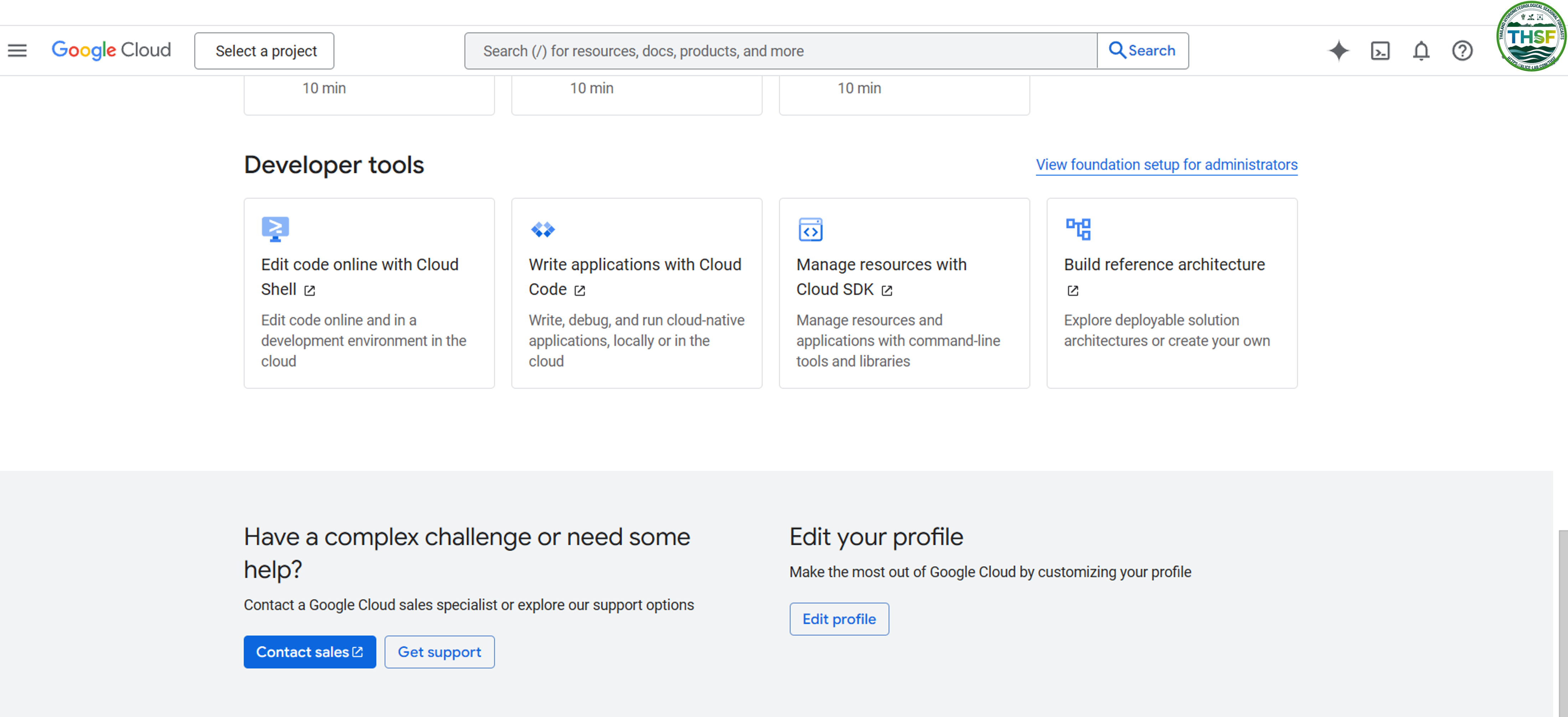
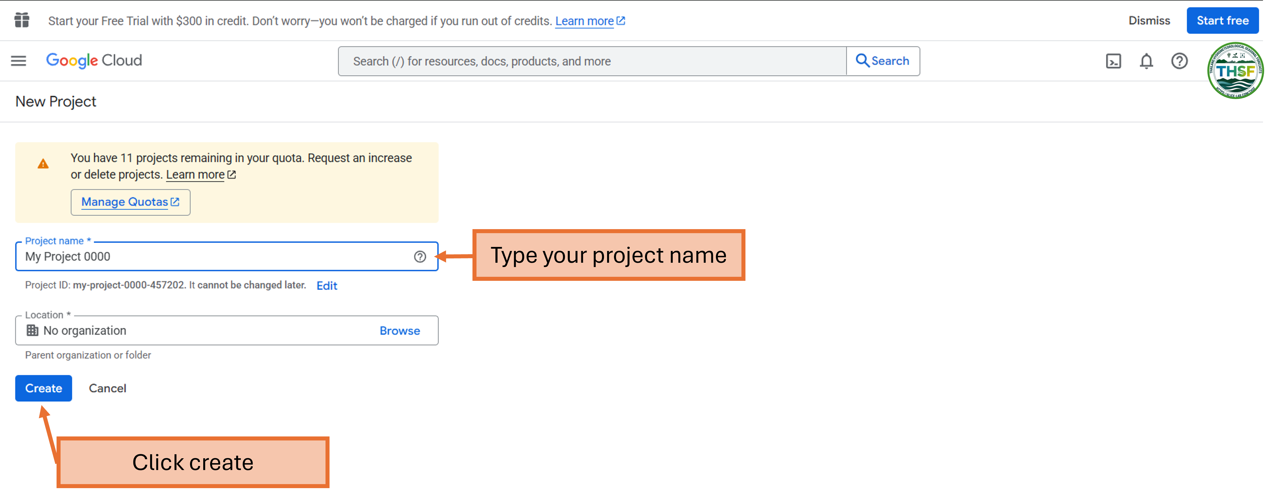
Create a Google Cloud Project:
- Go to Google Cloud Console

- Create a new project or use an existing one
- Create a new project and type your new project name:
- Enable the Earth Engine API for your project
- If your organisation restricts project creation, contact your IT administrators


Accessing the Earth Engine Platform
Once approved, you can access GEE through:
- Code Editor : The browser-based JavaScript IDE at code.earthengine.google.com
- Python API: For integrating GEE with Python workflows
- REST API: For custom applications and integration

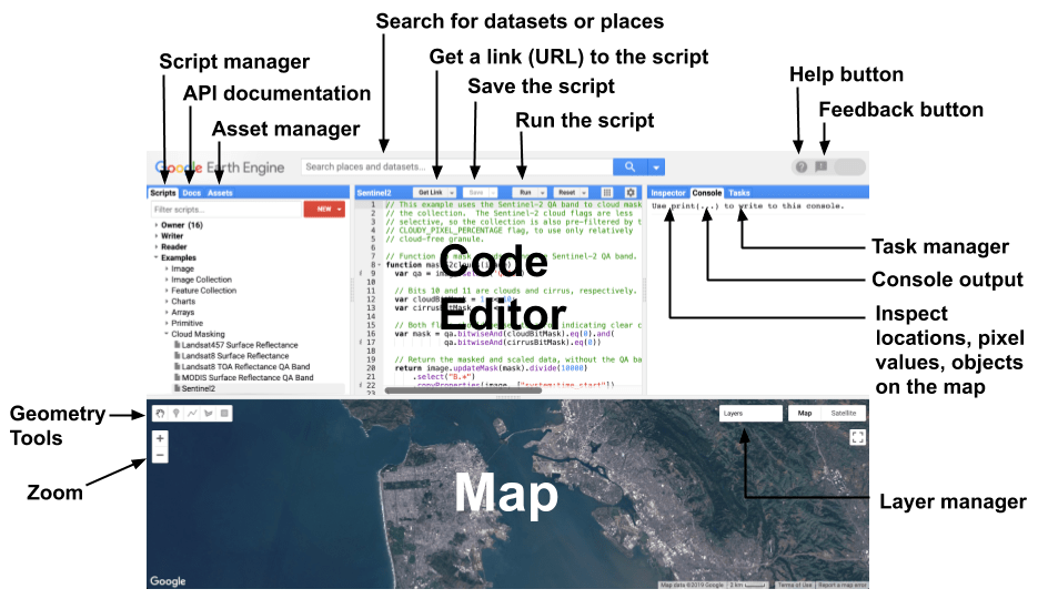
2. Exploring the Code Editor Interface
The Code Editor is the primary interface for most users. Here’s how to navigate it.
Main Components:
- Script Panel (left side) : Where you write JavaScript code
- Map Panel (center): Displays your visualisation results
- Console Panel (right side): Shows outputs, errors, and inspector results
- Asset Manager (top-left): Lists your imported and saved assets
- Documentation Panel (top-right): Shows function documentation

3. Working with Data in Earth Engine
Finding and Importing Datasets:
- Click on the “Datasets” tab in the Code Editor
- Browse categories or search for specific datasets
- Example: Search for “Landsat” to find Landsat collections
- Click on “Assets” in the left panel
- Use “New” → “Image Upload” or “Table Upload”
- You can also import data programmatically using the API
3.1 Explore the Data Catalog:
3.2 Import External Data:
4. Advanced Authentication and Project Management
Specifying a Cloud Project
For JavaScript users:
ee.initialize({projectId: 'my-project-id'
});
For Python users:
import ee
ee.Authenticate()
ee.Initialize(project='my-project-id')
5. Setting Up Python API AccessI
Install the Earth Engine Python API:
pip install earthengine-apiAuthenticate:
import ee
ee.Authenticate()
ee.Initialize()
By following this guide, you should be able to navigate Google Earth Engine’s powerful capabilities and start developing your own geospatial analysis projects.
🔍 Example on GEE:
GEE Code Editor

Google Earth Engine (GEE) – From Exploration to Export
Step 1: Explore & Visualize Data in GEE Code Editor
Access the Code Editor: Earth Engine Code Editor
Understanding the Code Editor Features
The GEE Code Editor is a web-based IDE for the Earth Engine JavaScript API, designed for geospatial analysis. It includes:
Step 2: Load data from project assets on Code Editor GEE
// Load temperature image from project assets
var temperature = ee.Image("projects/ee-udomporn/assets/AvgSurfT");
// Calculate statistics
var stats = temperature.reduceRegion({
  reducer: ee.Reducer.minMax(),
  geometry: temperature.geometry(),
  scale: 1000,
  bestEffort: true
});
// Print statistics
print("Min/Max:", stats);
print("Bands:", temperature.bandNames());
print("Resolution:", temperature.projection().nominalScale());
print("Projection:", temperature.projection());
print("Image Geometry:", temperature.geometry());
// Load Thailand boundary (Example: FAO GAUL dataset)
var thailand = ee.FeatureCollection('FAO/GAUL/2015/level0')
                .filter(ee.Filter.eq('ADM0_NAME', 'Thailand'));
});
Step 3: Select the band data and set for Visualization
// Select the first month of temperature data
var month1 = temperature.select('b1');
  palette: ['blue', 'cyan', 'yellow', 'orange', 'red']
// Visualization settings
var visParams = {
  min: 290,
  max: 315,
  palette: ['blue', 'cyan', 'yellow', 'orange', 'red']
Step 4: Display the map
// Display results on map
Map.centerObject(thailand, 6);
Map.addLayer(month1, visParams, 'Temperature');
Map.addLayer(thailand.style({color: 'black', width: 1}), {}, 'Boundary');
Map

Step 5: Select and clip for specific area
// Load Thailand Boundary Data (Level1 - Province)
var provinces = ee.FeatureCollection('FAO/GAUL/2015/level1')\
            .filter(ee.Filter.eq('ADM0_NAME', 'Thailand'))

// Filter Bangkok for example
var bangkok = provinces.filter(ee.Filter.eq('ADM1_NAME', 'Bangkok'))

// Clip the data by Bangkok Boundary
var bangkok_clipped = month1.clip(bangkok)

// Visualise the map
Map = geemap.Map(center=[13.7563, 100.5018], zoom=10)

// Add more details on the map
Map.centerObject(bangkok, 6);
Map.addLayer(bangkok_clipped, visParams, 'Temperature in Bangkok')

Step 6: Export Data to Google Drive
To save the clipped temperature data, we use Export.image.toDrive():
Export.image.toDrive({
  image: month1,
  description: 'Thailand_SurfaceTemp',
  folder: 'GEE',  // Creates a folder named "GEE" in Google Drive
  fileNamePrefix: 'AvgSurfT_Thailand',
  region: thailand.geometry(),
  scale: 1000,  // Resolution in metre
  crs: 'EPSG:4326',
  maxPixels: 1e13
Step 7: Running the Export Process
- Click "Tasks" tab.
- Click "Run" next to your export task.
- Wait for the process to finish—your image will be available in Google Drive.

Additional Notes
var month1 = temperature.select('b1').clip(thailand);
var month2 = temperature.select('b2').clip(thailand);
Google Colab – Using GEE Asset & Project
Step 1: Install Required Packages
To work with Google Earth Engine in Colab: Google Colab
# Install required packages
!pip install geemap rasterio localtileserver

Step 2: Import Libraries
import ee
import geemap
import os
from google.colab import drive
import matplotlib.pyplot as plt
import rasterio
from rasterio.plot import show
import numpy as np
Step 3: Connect Google Drive to Your Colab Session:
Google Colab does not have direct access to files, so we need to mount Google Drive:
# Mount Google Drive
drive.mount('/content/drive')
Grant Permissions


!ls /content/drive/MyDrive/
Step 4: Authenticate Earth Engine
Earth Engine requires authentication and initialisation before using its functions.
# Initialize Earth Engine
ee.Authenticate()


Step 5: Initialise Earth Engine with Your Project
# Initialize Earth Engine
ee.Initialize(project='ee-udomporn') # Your GEE Project Name
Step 6: Load Data from GEE Asset
# Load Data from GEE Asset
asset_id = "projects/ee-udomporn/assets/AvgSurfT"
temperature_image = ee.Image(asset_id)
Step 7: Check Min/Max for Each Band
To analyze the range of values for each band (month), loop through the bands and check their min/max values.
for i in range(1, 6):
    band_name = f'b{i}'
    stats = temperature_image.select(band_name).reduceRegion(
        reducer=ee.Reducer.minMax(),
        geometry=temperature_image.geometry(),
        scale=1000,  # Resolution in meters
        maxPixels=1e9
    ).getInfo()
    print(f'{band_name}: {stats}')
Step 8: Load Thailand Boundary
# Load Thailand Boundary from FAO GAUL
fao_admin = ee.FeatureCollection("FAO/GAUL_SIMPLIFIED_500m/2015/level1")

# Filter for Thailand
thailand = fao_admin.filter(ee.Filter.eq('ADM0_NAME', 'Thailand'))
Step 9: Select & Clip Data
# Extract Band 1 (Month 1)
month1 = temperature_image.select('b1')
Step 10: Visualize Data in geemap
Create an interactive map centered over Thailand.
Map = geemap.Map(center=[13, 101], zoom=6)

# Define visualization parameters
vis_params = {
    'min': 290,
    'max': 315,
    'palette': ['blue', 'cyan', 'yellow', 'orange', 'red']
}

# Create a style dictionary for a thin boundary line
thailand_outline = thailand.style(
    color='black',   # Line color
    width=0.5,       # Line width
    fillColor='00000000'  # Transparent fill color
)

# Add layers to the map
Map.addLayer(month1, vis_params, 'Surface Temp')
Map.addLayer(thailand_outline, {}, 'Thailand Boundary (Thin)')
Map.add_colorbar(vis_params, label='Temperature (K)')
Map.addLayerControl()

Map
Step 9: Clip Data to Specific Area
# Select Bangkok Boundary
bangkok = thailand.filter(ee.Filter.eq('ADM1_NAME', 'Bangkok'))

# Clip data to Bangkok Boundary
bangkok_clipped = month1.clip(bangkok)
# Visualise the result
Map.addLayer(bangkok_clipped, vis_params, 'Surface Temperature for Bangkok')  # มีศูนย์กลางที่กรุงเทพฯ

Map

Step 10: Export Data to Google Drive
# Export to Google Drive
task = ee.batch.Export.image.toDrive(
image=clipped_image,
description='Thailand_SurfaceTemp',
folder='GEE_Export', # Folder in your Google Drive
fileNamePrefix='AvgSurfT_Thailand',
region=thailand.geometry(),
scale=1000,
crs='EPSG:4326',
maxPixels=1e13
)
task.start()

print('Export Task Started. Check Earth Engine Tasks tab.')
AFTER export completed in GEE Task tab
# Download from Drive to Colab
!cp /content/drive/MyDrive/GEE_Export/AvgSurfT_Thailand.tif /content/

# Download to Local Computer
files.download('/content/AvgSurfT_Thailand.tif')
Final Workflow Summary
| Step | Process | Tool Used |
| 1 | Mount Google Drive | drive.mount('/content/drive') |
| 2 | Authenticate Earth Engine | ee.Authenticate() |
| 3 | Initialize Earth Engine with Project | ee.Initialize(project='your_project_name') |
| 4 | Load GEE Asset & Clip Data | ee.Image(asset_id), clip(thailand) |
| 5 | Check Min/Max for Each Band | reduceRegion() |
| 6 | Export Data to Google Drive | ee.batch.Export.image.toDrive() |
| 7 | Visualize Data in geemap | geemap.Map() |
| 8 | Download to Local Computer | files.download() |
Important Notes
🔍 Link to Example code : Google Colab
Working with Google Earth Engine for Geospatial Analysis
This tutorial shows how to analyse and visualise geospatial temperature data using Google Earth Engine (GEE) and Python. We’ll cover authentication, loading Earth Engine assets, processing data, and creating interactive maps.
Step-By-Step Earth Engine Workflow in Python
Step 1. install geemap and library
!pip install geemap earthengine-api
Step 2. Authenticate Earth Engine
import ee

# Authenticate
ee.Authenticate()
Step 3. Initialize Earth Engine with Your Project
# Initialize Earth Engine with your specific project
ee.Initialize(project='ee-udomporn')  # Replace with your GEE Project Name
Step 4. Load Data from GEE Asset
# Load temperature data from your Earth Engine asset
asset_id = "projects/ee-udomporn/assets/AvgSurfT"
temperature_image = ee.Image(asset_id)

# Print basic information about the image
print(temperature_image.bandNames().getInfo())
Step 5. Check Min/Max for Each Band
# Function to get min/max values for a band
def get_band_stats(image, band_name):
    stats = image.select(band_name).reduceRegion(
        reducer=ee.Reducer.minMax(),
        geometry=image.geometry(),
        scale=1000,
        maxPixels=1e9
    )
    return stats.getInfo()

# Get band names
band_names = temperature_image.bandNames().getInfo()

# Print stats for each band
for band in band_names:
    stats = get_band_stats(temperature_image, band)
    print(f"แบนด์ {band}: ต่ำสุด = {stats[band+'_min']}, สูงสุด = {stats[band+'_max']}")
Step 6. Load Thailand Boundary from FAO GAUL
# Load Thailand boundary from FAO's Global Administrative Unit Layers
thailand = ee.FeatureCollection('FAO/GAUL/2015/level0')\
           .filter(ee.Filter.eq('ADM0_NAME', 'Thailand'))

# Print information about the boundary
print(f"Thailand boundary: {thailand.first().getInfo()['properties']['ADM0_NAME']}")
Step 7. Visualise Data in GeeMap
import geemap

# Create a map centered on Thailand
Map = geemap.Map(center=[13, 101], zoom=6)

# Define visualization parameters
vis_params = {
    'min': 290,
    'max': 315,
    'palette': ['blue', 'cyan', 'yellow', 'orange', 'red']
}

# Create a style dictionary for a thin boundary line
thailand_outline = thailand.style(
    color='black',   # Line color
    width=0.5,       # Line width
    fillColor='00000000'  # Transparent fill color
)

# Add layers to the map
Map.addLayer(clipped_image, vis_params, 'Thailand Surface Temperature')
Map.addLayer(thailand_outline, {}, 'Thailand Boundary (Thin)')
Map.add_colorbar(vis_params, label='Temperature (K)')
Map.addLayerControl()

# Display the map
Map
Step 8. Selecting & Clipping Data to Bangkok Boundary
# Load Thailand admin level 1 (province) boundaries
provinces = ee.FeatureCollection('FAO/GAUL/2015/level1')\
            .filter(ee.Filter.eq('ADM0_NAME', 'Thailand'))

# Filter to get only Bangkok
bangkok = provinces.filter(ee.Filter.eq('ADM1_NAME', 'Bangkok'))

# Print the name to verify
print(f"Selected area: {bangkok.first().getInfo()['properties']['ADM1_NAME']}")

# Select Band 1 (Month 1)
month1 = temperature_image.select('b1')

# Clip image to Bangkok boundary
bangkok_clipped = month1.clip(bangkok)
Step 9. Visualising Bangkok Temperature Data
# Create a map centered on Bangkok
Map = geemap.Map(center=[13.7563, 100.5018], zoom=10)  # Centered on Bangkok

# Define visualization parameters
vis_params = {
    'min': 290,
    'max': 315,
    'palette': ['blue', 'cyan', 'yellow', 'orange', 'red']
}

# Create a style dictionary for a thin boundary line
bangkok_outline = bangkok.style(
    color='black',   # Line color
    width=1,         # Line width
    fillColor='00000000'  # Transparent fill color
)

# Add layers to the map
Map.addLayer(bangkok_clipped, vis_params, 'Bangkok Surface Temperature')
Map.addLayer(bangkok_outline, {}, 'Bangkok Boundary')
Map.add_colorbar(vis_params, label='Temperature (K)')
Map.addLayerControl()

# Display the map
Map

Step 10. Exporting Earth Engine Data to Your Local Drive
# Export PNG
Map.to_image('bangkok_temperature_map.png')
print("ส่งออกแผนที่เป็น PNG สำเร็จแล้ว")
# Export JPG
Map.to_jpg('bangkok_temperature_map.jpg')
print("Exported JPG file successfully")
# Export PDF
Map.to_pdf('bangkok_temperature_map.pdf')
print("Exported PDF file successfully")
import os

# set directory to save the file
output_dir = './exports'
if not os.path.exists(output_dir):
    os.makedirs(output_dir)

# set the path for file
output_file = os.path.join(output_dir, 'bangkok_temp.tif')

# export GeoTIFF
geemap.ee_export_image(
    bangkok_clipped,  # image
    filename=output_file,  # file name
    scale=100,  # resolution
    region=bangkok.geometry(),  # boundary
    file_per_band=False
)
print(f"Exported to {output_file} successfully")
By combining Earth Engine’s cloud processing capabilities with local file access, you can efficiently analyse geospatial data while maintaining the flexibility of your local development environment.
🔍 Link to Download Jupyter Notebook: Jupyter Notebook
Reading Spatial Data in Python
Working with geospatial data locally offers numerous advantages including faster processing, enhanced privacy, and the ability to work without an internet connection. This guide focuses on two critical spatial data formats: GeoTIFF and NetCDF files, providing comprehensive instructions for setting up your environment, loading data, visualization techniques, and advanced spatial operations.
Whether you’re analysing remote sensing imagery, climate data, or creating specialised maps, these step-by-step instructions will help you build a robust offline geospatial workflow in Python. By the end of this guide, you’ll be able to confidently manipulate spatial data, create informative visualisations, and perform common geographic operations such as clipping to specific regions.
- Python Setup
- Reading GeoTiff
- Reading NetCDF
Geospatial Python Environment Setup (Windows)
This guide will walk you through setting up a complete geospatial Python environment on Windows, with all the essential libraries for geospatial data analysis, visualisation, and processing.
Step 1. Install Anaconda (Python 3.10 recommended)
Go to: Anaconda Download
Download the Windows installer (64-bit) for Python 3.10
- Run the installer:
- Download the Windows installer (64-bit) for Python 3.10
- Run the installer:
Step 2. Create a New Conda Environment (geo_env)
- Open Anaconda Prompt (search it from Start Menu)
- Run the following commands:
conda create -n geo_env python=3.10
conda activate geo_env
Step 3. Install Required GeoPython Packages
conda install -c conda-forge rasterio geopandas xarray geemap localtileserver jupyterlab notebook earthengine-api ipykernel
Step 4. Add geo_env to Jupyter Notebook Kernels
python -m ipykernel install --user --name=geo_env --display-name "Python (geo_env)"
Step 5. Launch Jupyter Notebook
jupyter notebook
✅ Test Your Setup
import rasterio
import geemap
print("Everything is working ✅")
📌 Notes
conda activate geo_env
jupyter notebook
Step 6. Troubleshooting Common Issues
conda install -c conda-forge rasterio
conda install -c conda-forge geopandas
conda install -c conda-forge xarray
# and so on...
conda install -c conda-forge gdal
Memory Errors During Installation
Python Version Conflicts
conda create -n geo_env python=3.9 # หรือเวอร์ชันอื่น
Updating Your Environment
conda update --all
pip install rasterio geopandas xarray geemap
Additional Useful Packages
conda install -c conda-forge matplotlib seaborn plotly contextily folium rasterstats
🔗 Extra: Setting Up Google Earth Engine Authentication
If you’re using Google Earth Engine (GEE), you’ll need to authenticate:
import ee
ee.Authenticate()  # ทำตามคำแนะนำในเบราว์เซอร์ของคุณ
ee.Initialize()
This concludes our comprehensive guide on reading, processing, and visualizing spatial data in Python. By following these techniques, you can effectively work with both GeoTIFF and NetCDF data formats offline, enabling sophisticated geospatial analysis even without internet connectivity.
GeoTIFF Data Handling and Visualisation
This tutorial demonstrates how to work with GeoTIFF data offline using Python. You’ll learn how to download, read, visualise, and manipulate geospatial raster data – all while working locally on your machine.
This approach is ideal for environments with limited internet connectivity or when working with large datasets.
Prerequisites – – Verify Package Installation
# Test importing each package
import rasterio
import geopandas
import matplotlib
import numpy
import requests

print("All packages imported successfully!")
Tutorial Workflow
Step 1. Download GeoTIFF from Our Platform and Save Locally
First, let’s download a sample GeoTIFF file and save it to your local machine. There are two ways:
1. Download directly from our platform

2. Download using python code
import requests

# Direct download link from the platform
url = "https://dl.dropboxusercontent.com/scl/fi/ijfjpdntc1qv068wjlbbb/AvgSurfT.tif?rlkey=wx9lgdgkcf2ahrymemln1y37v&dl=0"
output_path = "AvgSurfT.tif"

# Download and save locally
response = requests.get(url)
with open(output_path, "wb") as f:
    f.write(response.content)

print("File downloaded and saved as:", output_path)
Step 2. Read the GeoTIFF and Explore Its Properties
import rasterio

# Open the GeoTIFF file
with rasterio.open("AvgSurfT.tif") as dataset:
    print("Metadata:", dataset.profile)
    print("CRS:", dataset.crs)
    print("Number of bands:", dataset.count)
Step 3. Read Band Data and Compute Statistics
import numpy as np

with rasterio.open("AvgSurfT.tif") as dataset:
    band1 = dataset.read(1).astype("float64")  # Read first band
    valid_data = band1[~np.isnan(band1)]  # Mask NaNs

    stats = {
        'min': float(np.min(valid_data)),
        'max': float(np.max(valid_data)),
        'mean': float(np.mean(valid_data)),
        'std': float(np.std(valid_data))
    }

    print("Band 1 Statistics:", stats)
Step 4. Visualise Band Data with a Colormap
import matplotlib.pyplot as plt

plt.figure(figsize=(6, 8))
plt.imshow(band1, cmap='hot_r', vmin=280, vmax=320)
plt.colorbar(label="Temperature (K)")
plt.title("AvgSurfT - Band 1")
plt.xlabel("X (pixels)")
plt.ylabel("Y (pixels)")
plt.show()

Step 5. Replace Pixel Coordinates with Geographic Coordinates
with rasterio.open("AvgSurfT.tif") as src:
    band1 = src.read(1)
    transform = src.transform

    from rasterio.transform import xy

    # Get dimensions
    nrows, ncols = band1.shape

    # Get lon/lat of top-left and bottom-right
    lon_min, lat_max = xy(transform, 0, 0)
    lon_max, lat_min = xy(transform, nrows - 1, ncols - 1)

    # Create extent
    extent = [lon_min, lon_max, lat_min, lat_max]

plt.figure(figsize=(10, 6))
plt.imshow(band1, cmap='hot_r', vmin=280, vmax=320, extent=extent)
plt.colorbar(label="Temperature (K)")
plt.title("AvgSurfT - Band 1")
plt.xlabel("Longitude")
plt.ylabel("Latitude")
plt.show()

Step 6. Plot All Bands
# Open the dataset
with rasterio.open("AvgSurfT.tif") as dataset:
    num_bands = dataset.count  # Number of bands
    transform = dataset.transform
    height = dataset.height
    width = dataset.width

    # Get the geographic extent
    lon_min, lat_max = xy(transform, 0, 0)
    lon_max, lat_min = xy(transform, height - 1, width - 1)
    extent = [lon_min, lon_max, lat_min, lat_max]

    # Create subplots for each band
    fig, axes = plt.subplots(1, num_bands, figsize=(5 * num_bands, 6))

    if num_bands == 1:
        axes = [axes]  # Ensure axes is always iterable

    for i in range(num_bands):
        band = dataset.read(i + 1)  # Read band (1-based index)
        ax = axes[i]
        im = ax.imshow(band, cmap='hot_r', vmin=280, vmax=320, extent=extent)
        ax.set_title(f"Band {i + 1}")
        ax.set_xlabel("Longitude")
        ax.set_ylabel("Latitude")
        plt.colorbar(im, ax=ax, shrink=1)

    plt.tight_layout()
    plt.show()

Step 7. Clip the GeoTIFF to a Region (Thailand Boundary)
import geopandas as gpd
from rasterio.mask import mask

# Load the GADM level-1 shapefile for Thailand
thailand = gpd.read_file("path/to/your/shapefile.shp")  # Update with your path

# Clip only to a specific province
bangkok = thailand[thailand["shapeName"] == "Bangkok"]

# Open GeoTIFF and perform clipping
with rasterio.open("AvgSurfT.tif") as src:
    if bangkok.crs != src.crs:
        bangkok = bangkok.to_crs(src.crs)

    # Clip the raster
    out_image, out_transform = mask(src, bangkok.geometry, crop=True)
    out_meta = src.meta.copy()

    # Update metadata for output
    out_meta.update({
        "height": out_image.shape[1],
        "width": out_image.shape[2],
        "transform": out_transform
    })
Step 8. Save and Visualize the Clipped Output
# Save clipped GeoTIFF
with rasterio.open("AvgSurfT_bkk.tif", "w", **out_meta) as dest:
    dest.write(out_image)

# Get number of rows and columns
nrows, ncols = out_image.shape[1], out_image.shape[2]

# Get the bounding coordinates using the affine transform
lon_min, lat_max = xy(out_transform, 0, 0)
lon_max, lat_min = xy(out_transform, nrows - 1, ncols - 1)

# Create extent for imshow (left, right, bottom, top)
extent = [lon_min, lon_max, lat_min, lat_max]

# Plot raster and boundary
fig, ax = plt.subplots(figsize=(10, 6))
raster = ax.imshow(out_image[0], cmap='hot_r', vmin=300, vmax=320, extent=extent)
bangkok.boundary.plot(ax=ax, edgecolor='black', linewidth=0.5)
plt.colorbar(raster, ax=ax, label="Temperature (K)")
ax.set_title("AvgSurfT - Clipped to Bangkok with Boundary")
ax.set_xlabel("Longitude")
ax.set_ylabel("Latitude")
ax.set_axis_on()
plt.savefig("AvgSurfT_bkk_with_boundary.png", dpi=300)
plt.show()

Conclusion
This tutorial has demonstrated how to work with GeoTIFF data offline using Python. You’ve learned how to:
This concludes our comprehensive guide on reading, processing, and visualizing spatial data in Python. By following these techniques, you can effectively work with both GeoTIFF and NetCDF data formats offline, enabling sophisticated geospatial analysis even without internet connectivity.
🔍 Click to download example : GeoTiff in Python
Processing and Visualising NetCDF Data
This guide provides comprehensive instructions for working with NetCDF (.nc) files in Python, including data loading, analysis, and creating various visualisations with a focus on meteorological and geospatial data.
Prerequisites — Download NetCDF file from our platform:

Step 1. Installation of Required Libraries
pip install xarray netCDF4 matplotlib numpy scipy cartopy geopandas
Step 2. Loading and Exploring NetCDF Data
import xarray as xr
import os
import matplotlib.pyplot as plt
import geopandas as gpd
import numpy as np
import pandas as pd

# Path to your NetCDF file
nc_file_path = r"C:\Users\ASUS\Jupyter\ALICE\data\AvgSurfT.nc"

# Open the dataset
ds = xr.open_dataset(nc_file_path)

# Explore the dataset structure
print("Dataset overview:")
print(ds)

# View available variables in the dataset
print(f"Available variables: {list(ds.data_vars)}")

# Extract the variable of interest
var_data = ds['AvgSurfT']  # Replace with your variable name if different

# Examine metadata and attributes
print(f"Variable attributes: {var_data.attrs}")
print(f"Dimensions: {var_data.dims}")
print(f"Coordinates: {var_data.coords}")
print(f"Shape: {var_data.shape}")
Step 3. Basic Statistics and Data Exploration
# Calculate basic statistics
ds_mean_value = var_data.mean().values
ds_min_value = var_data.min().values
ds_max_value = var_data.max().values
ds_std_dev = var_data.std().values
# Get time range
min_date = str(var_data.time.values.min())[:10]
max_date = str(var_data.time.values.max())[:10]

# Display statistics
print(f"Time range: {min_date} to {max_date}")
print(f"Mean: {ds_mean_value:.4f} {var_data.attrs.get('units', '')}")
print(f"Min: {ds_min_value:.4f} {var_data.attrs.get('units', '')}")
print(f"Max: {ds_max_value:.4f} {var_data.attrs.get('units', '')}")
print(f"Std Dev: {ds_std_dev:.4f} {var_data.attrs.get('units', '')}")

# Additional spatial statistics
print("\nSpatial Analysis:")
spatial_mean = var_data.mean(dim=['lat', 'lon']).values
print(f"Mean across all locations: {spatial_mean.mean():.4f}")

# Temporal statistics
print("\nTemporal Analysis:")
if 'time' in var_data.dims:
    temporal_mean = var_data.mean(dim='time')
    print(f"Mean temporal value shape: {temporal_mean.shape}")
    print(f"Max value in temporal mean: {temporal_mean.max().values:.4f}")
    print(f"Min value in temporal mean: {temporal_mean.min().values:.4f}")
# Spatial Visualisation with Geographic Boundaries
# Load Thailand boundary
thailand_boundary = gpd.read_file("https://geodata.ucdavis.edu/gadm/gadm4.1/json/gadm41_THA_0.json")

# Create a figure with two subplots
fig, axes = plt.subplots(1, 2, figsize=(14, 6), constrained_layout=True)

# Historical spatial average (left subplot)
temp = ds  # Using the original dataset
temp['AvgSurfT'].mean(dim="time").plot(
    cmap="hot_r", ax=axes[0], vmin=290, vmax=310,
    cbar_kwargs={"label": "Historical AvgSurfT (K)"}
)
thailand_boundary.plot(edgecolor="black", facecolor="none", lw=0.7, ax=axes[0])
axes[0].set_title(f"Historical AvgSurfT\n{min_date} to {max_date}")
axes[0].set_xlabel("Longitude")
axes[0].set_ylabel("Latitude")


# Standard deviation plot (right subplot)
temp['AvgSurfT'].std(dim="time").plot(
    cmap="viridis", ax=axes[1],
    cbar_kwargs={"label": "AvgSurfT Standard Deviation (K)"}
)
thailand_boundary.plot(edgecolor="black", facecolor="none", lw=0.7, ax=axes[1])
axes[1].set_title(f"AvgSurfT Variability\n{min_date} to {max_date}")
axes[1].set_xlabel("Longitude")
axes[1].set_ylabel("Latitude")
# Save plot
fig.savefig(r"C:\Users\ASUS\Jupyter\ALICE\data\AvgSurfT\ncAvgSurfT_map.png", dpi=300, bbox_inches='tight')
plt.show()
Step 5. Multiple Time Step Visualisation
# Get the number of available time steps
time_steps = len(var_data.time)

# Determine how many to plot (up to 6)
n_plots = min(time_steps, 6)

# Create a 1xn subplot
fig, axes = plt.subplots(nrows=1, ncols=n_plots, figsize=(4*n_plots, 4), constrained_layout=True)

# If only one subplot, make axes iterable
if n_plots == 1:
    axes = [axes]

# Plot each time step in its subplot
for i, time_idx in enumerate(range(n_plots)):
    ax = axes[i]
    time_value = var_data.time.values[time_idx]
    time_data = var_data.sel(time=time_value)

    # Plot temperature and overlay boundary
    time_data.plot(ax=ax, cmap="hot_r", vmin=280, vmax=315,
                  cbar_kwargs={'label': '' if i < n_plots-1 else 'AvgSurfT (K)'})  # Only last plot shows colorbar label
    thailand_boundary.plot(ax=ax, edgecolor="black", facecolor="none", linewidth=0.7)

    # Format time string for title
    time_str = str(time_value)[:10]  # Get YYYY-MM-DD format
    ax.set_title(f"{time_str}")
    ax.set_xlabel("")
    ax.set_ylabel("" if i > 0 else "Latitude")

    # Add longitude label only to the bottom plots
    if i == n_plots // 2:
        ax.set_xlabel("Longitude")

# Global title
plt.suptitle(f"AvgSurfT Maps ({min_date} to {max_date})", fontsize=16, y=1.05)

# Save the plot
plt.savefig(r"C:\Users\ASUS\Jupyter\ALICE\data\AvgSurfT\ncAvgSurfT_allmap.png", dpi=300, bbox_inches='tight')
plt.show()
Step 6. Clip the NetCDF to a Region (Bangkok Boundary)
import rioxarray as rio

# Ensure NetCDF data has proper spatial dimensions and CRS
ds_geo = temp['AvgSurfT'].rio.set_spatial_dims(x_dim="lon", y_dim="lat")
ds_geo = ds_geo.rio.write_crs("EPSG:4326")  # Set to WGS84 coordinate system

# Filter GeoDataFrame to select only Bangkok
thailand_boundary = gpd.read_file("https://geodata.ucdavis.edu/gadm/gadm4.1/json/gadm41_THA_1.json")
bangkok = thailand_boundary[thailand_boundary["NAME_1"].isin(["BangkokMetropolis"])]

# Check that the boundary is in the correct CRS
if bangkok.crs != "EPSG:4326":
    bangkok = bangkok.to_crs("EPSG:4326")

# Clip the NetCDF data to the Bangkok boundary
bangkok_data = ds_geo.rio.clip(bangkok.geometry, bangkok.crs)

# Calculate temporal mean for visualization
bangkok_mean = bangkok_data.mean(dim='time')

# Visualize the clipped data
plt.figure(figsize=(10, 8))
im = bangkok_mean.plot(cmap='hot_r', vmin=300, vmax=315, add_colorbar=False)  # Remove default color bar
plt.colorbar(im, shrink=0.8)  # Add custom-sized color bar (adjust shrink value as needed)
bangkok.boundary.plot(edgecolor='black', linewidth=1.5, ax=plt.gca())
plt.title(f"Average Surface Temperature in Bangkok\n{min_date} to {max_date}")
plt.xlabel("Longitude")
plt.ylabel("Latitude")
plt.tight_layout()

# Save the clipped data if needed
plt.savefig("Bangkok_AvgSurfT.png", dpi=300, bbox_inches='tight')
plt.show()
Summary and Conclusion
When working with NetCDF (.nc) files in Python, remember these key steps:
1. Initial Exploration: Open the file with xarray and examine its structure, variables, and dimensions.
2. Data Extraction: Select the specific variables and regions of interest from the dataset.
3. Statistical Analysis: Calculate basic statistics and perform temporal/spatial analysis.
4. Visualisation: Create meaningful plots to visualise your data (time series, maps, etc.).
5. Data Export: Save processed data and results in appropriate formats.
By following this guide, you should be able to effectively process, analyse, and visualise data from NetCDF files for meteorological, climate, and geospatial applications.
Remember to always check the coordinate systems, units, and metadata of your NetCDF files, as these can vary depending on the source and type of data.
🔍 To download the python script please click: NetCDF in Python
How to read/process/plot time series data using Python
Time series data is essential for tracking changes over time—whether it’s climate measurements, hydrological trends, or environmental indicators. In geospatial workflows, we often work with time series from different sources such as Google Earth Engine (GEE) or Excel spreadsheets.
This guide walks you through two practical workflows to handle time series data using Python:
1. From Google Earth Engine to Python
2. From Excel-based datasets (e.g., basin or district-level stats)
- From Google Earth Engine to Python
- From Excel-based datasets to Python
Read Time Series Data from GEE into Python
Google Earth Engine (GEE) is a powerful platform for analysing geospatial data. It allows users to store, process, and visualise satellite imagery and other geospatial datasets. Sometimes, you may export time series data (e.g., climate, land use, temperature) from GEE as a FeatureCollection (table format). This guide walks you through how to read and analyze that time series table data in Python using earthengine-api and pandas.
Whether you’re tracking surface temperature over time or rainfall across basins, this guide gives you the tools to process and visualize it with ease.
Step 1. Install Required Libraries
pip install earthengine-api pandas matplotlibOptional: If using Jupyter, also install ipython, notebook, or jupyterlab.
Step 2. Authenticate and Initialize Earth Engine
import ee

# First-time authentication
ee.Authenticate()

# Initialize the Earth Engine API
ee.Initialize()
Step 3. Load Your GEE Table Asset (Time Series Data)
asset_path = "projects/ee-udomporn/assets/AvgSurfT_basin"
basin_fc = ee.FeatureCollection(asset_path)
Step 4. Convert to pandas DataFrame
features = basin_fc.getInfo()['features']
records = [f['properties'] for f in features]

basin_df = pd.DataFrame(records)
Step 5. Parse Dates and Set Time Index
# Convert to datetime and set index
basin_df['Date'] = pd.to_datetime(basin_df[['Year', 'Month', 'Day']])
basin_df.set_index('Date', inplace=True)

# Optional: remove separate date parts
basin_df.drop(columns=['Day', 'Month', 'Year'], inplace=True, errors='ignore')
Step 6. Explore Statistics
# Select only numeric columns
numeric_data = basin_df.select_dtypes(include='number')

# Basic stats
stats = pd.DataFrame({
    'Mean (K)': numeric_data.mean(),
    'Min (K)': numeric_data.min(),
    'Max (K)': numeric_data.max(),
    'Std Dev (K)': numeric_data.std()
}).round(2)

print(stats)
stats['Mean (K)'].sort_values().plot(kind='barh', figsize=(10, 6), color='skyblue')
plt.title('Average Surface Temperature by Basin')
plt.xlabel('Temperature (K)')
plt.grid(True)
plt.tight_layout()
plt.show()
Step 7. Visualise Time Series (Example)
import matplotlib.pyplot as plt

plt.figure(figsize=(10, 4))
plt.plot(basin_df.index, basin_df['Chi'], label='Chi Basin', color='tab:blue')
plt.title('Surface Temperature - Chi Basin')
plt.xlabel('Date')
plt.ylabel('AvgSurfT (K)')
plt.grid(True)
plt.legend()
plt.tight_layout()
plt.show()

basins = ['Chi', 'Mun', 'Ping']
fig, axes = plt.subplots(1, 3, figsize=(18, 4), constrained_layout=True)

for i, basin in enumerate(basins):
    axes[i].plot(basin_df.index, basin_df[basin], label=basin)
    axes[i].set_title(basin)
    axes[i].set_xlabel('Date')
    axes[i].set_ylabel('AvgSurfT (K)')
    axes[i].grid(True)

plt.suptitle('AvgSurfT - Selected Basins')
plt.show()

Step 8. Saving Processed Data
# Save the processed data to a new Excel file
output_path = "processed_basin_data.xlsx"
basin_df.to_excel(output_path)
print(f"Processed data saved to {output_path}")

# Save plots as image files
fig.savefig("basin_plot.png", dpi=300, bbox_inches='tight')
print("Plot saved as image file")
Conclusion
You’ve now learned how to:
🔍 Download the example: GEE into Python
Processing and Visualising Time Series Data from Excel
This guide will walk you through the process of reading, processing, and visualising time series data from Excel files using Python. We’ll cover installation of necessary libraries, data loading, preprocessing, statistical analysis, and creating various visualizations.
Prerequisites — Download Excel file from our platform:

Step 1. Installation of Required Libraries
pip install pandas matplotlib numpy scipy seaborn openpyxl
Step 2. Loading Data from Excel
import pandas as pd
import matplotlib.pyplot as plt
import numpy as np
import seaborn as sns
from scipy import stats

# Set the path to your Excel file
basin_excel_path = r"C:\data\AvgSurfT\AvgSurfT_basin.xlsx"

# Preview the data
basin_df = pd.read_excel(basin_excel_path)
print(basin_df.head())  # Display the first 5 rows
print(basin_df.columns)  # Display column names

# Re-read the Excel file, skipping the first row (for Thai column headers)
basin_df = pd.read_excel(basin_excel_path, skiprows=1)
print(basin_df.columns)  # Display column names after skipping first row
Step 3. Data Preprocessing
# Convert date-related columns to integers
basin_df['Year'] = basin_df['Year'].astype(int)
basin_df['Month'] = basin_df['Month'].astype(int)
basin_df['Day'] = basin_df['Day'].astype(int)

# Convert to datetime and set as index
basin_df['Date'] = pd.to_datetime(basin_df[['Year', 'Month', 'Day']])
basin_df.set_index('Date', inplace=True)

# Drop original date columns if desired
basin_df.drop(columns=['Year', 'Month', 'Day'], inplace=True)

# Check the processed data
print(basin_df.info())
print(basin_df.describe())
Step 4. Exploratory Data Analysis
# Check for missing values
print("\nMissing values in each column:")
print(basin_df.isna().sum())

# Basic statistics for each basin
print("\nBasic statistics:")
print(basin_df.describe())

# Check the temporal coverage
print("\nData spans from:", basin_df.index.min(), "to", basin_df.index.max())

# Check for outliers using Z-score
z_scores = stats.zscore(basin_df)
potential_outliers = (abs(z_scores) > 3).any(axis=1)
print("\nNumber of potential outliers:", potential_outliers.sum())

# Monthly and seasonal patterns
basin_df['Month'] = basin_df.index.month
basin_df['Year'] = basin_df.index.year

# Calculate monthly averages
monthly_avg = basin_df.groupby('Month').mean()
print("\nMonthly averages:")
print(monthly_avg)

# Remove the added columns if you don't need them anymore
basin_df.drop(columns=['Month', 'Year'], inplace=True, errors='ignore')
Step 5. Basic Visualisations
plt.figure(figsize=(10, 4))
plt.plot(basin_df.index, basin_df['Chi'], color='tab:blue')
plt.title('AvgSurfT - Chi Basin')
plt.xlabel('Date')
plt.ylabel('AvgSurfT (K)')
plt.grid(True)
plt.tight_layout()
plt.show()
basins_to_plot = ['Chi', 'Mun', 'Ping']
fig, axes = plt.subplots(nrows=1, ncols=3, figsize=(18, 4), sharey=True)

for i, basin in enumerate(basins_to_plot):
    axes[i].plot(basin_df.index, basin_df[basin], label=basin, color=f'tab:{["blue", "orange", "green"][i]}')
    axes[i].set_title(f'{basin} Basin')
    axes[i].set_xlabel('Date')
    axes[i].grid(True)

axes[0].set_ylabel('AvgSurfT (K)')
plt.suptitle('AvgSurfT - Selected Basins', fontsize=16)
plt.tight_layout(rect=[0, 0, 1, 0.95])
plt.show()
Step 6. Saving Processed Data
# Save the processed data to a new Excel file
output_path = "processed_basin_data.xlsx"
basin_df.to_excel(output_path)
print(f"Processed data saved to {output_path}")

# Save plots as image files
fig.savefig("basin_plot.png", dpi=300, bbox_inches='tight')
print("Plot saved as image file")
By following this comprehensive guide, you can effectively process, analyse, and visualise time series data from Excel files using Python. The techniques demonstrated can be applied to various types of time series data, not just surface temperature measurements.
🔍 To download the python script please click: Python Time series